Chapter 1 · Meet the DMP: a recipe for movement
You will meet the spring, push and clock that let a robot repeat one motion toward new goals.
Imagine guiding a robot arm by hand as it lifts a cup onto a shelf, showing it a graceful curve just once. Then someone moves the shelf 20 cm to the left, and the arm carries the cup to the new spot with the same smooth motion, without another lesson. How does it do that?
The answer is a small recipe called a dynamic movement primitive, or DMP, whose three ingredients we will meet along the way. By the end of this chapter, you will be able to describe that recipe in one sentence.
The picture
Picture yourself walking a dog home, with the leash gently drawing it toward your front door. That pull is the spring: it always points home, and the farther the dog wanders, the harder it pulls.
Along the way, a puddle spreads across the sidewalk, so you give the leash a little sideways tug to steer the dog around it. That tug is the push, shaping the route you take while leaving your destination alone.
Because the puddle is always a few minutes into the walk, a glance at your watch tells you when the tug is coming. Your watch is the clock.
Now swap the dog for a robot hand and the front door for a shelf, and you have the picture behind a DMP. In Figure 1, those same three parts become boxes that feed one moving dot.


The idea
With that walk in mind, we can give each part a job in the robot’s motion. The spring pulls the hand toward a goal, the place where the motion should end, and makes sure it arrives. The push is the learned nudge you taught by hand, bending the path into the shape you showed.
Meanwhile, the clock slowly runs down from 1 toward 0, telling the push when to act and letting it fade out as the motion comes to an end.
Put those ingredients together and you have your one-sentence recipe: a DMP is a spring that pulls toward a goal, plus a learned push that shapes the path, plus a clock that tells the push when to act.
Intuition: the goal lives in the spring
The push stores the shape of the motion, while the spring stores the place where it ends, which means you can move the goal without touching what you taught. The spring pulls somewhere new, and the push keeps bending the path in the way you showed.
Now the shelf puzzle has an answer: once the robot has learned the push, moving the shelf only changes the goal.
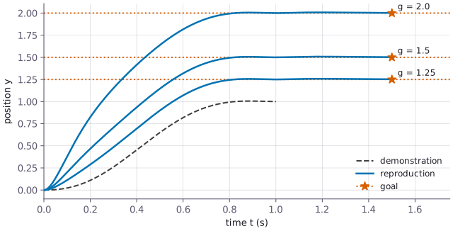
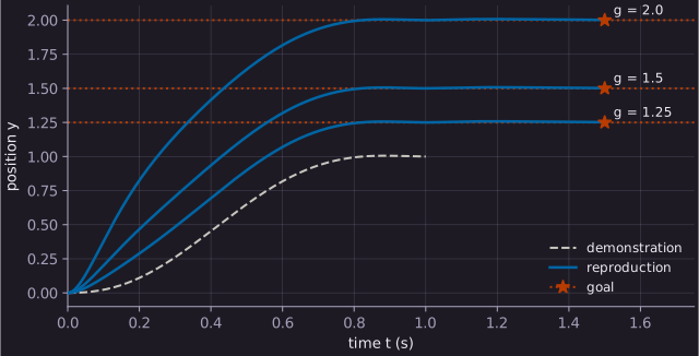
You can follow that story in Figure 2, where the dashed demonstration ends at a goal of 1.0. The three solid lines replay it toward three new goals, each marked with a star, and every path reaches its star even though the robot was never shown those destinations.
The math
Each of our three ingredients has a short equation, and here you get a first glimpse of them together. We will open these boxes one by one in the coming chapters, so you can let the details wait.
Intuition: a spring with a nudge
Picture a ball attached to a spring hooked to the goal: when you let go, it swings home. Add a gentle hand to nudge it along the way, and you have the picture that the three equations below put into words and symbols.
Before we look inside, let’s give those moving parts their names: the robot’s position is \(\krepro{y}\). Its helper variable \(\krepro{z}\) is the velocity scaled by the time constant \(\kphase{\tau}\), which we will explore in Chapter 2. The destination is our goal \(\kgoal{g}\), while the clock value is the phase \(\kphase{x}\), starting at 1 and decaying toward 0. Along the route, the push \(\kforce{f(x)}\) shapes the motion.
The math: eq. (1)–(3)
\[ \kphase{\tau}\,\krepro{\dot z} = \underbrace{\kspring{\alpha_z\big(\beta_z(\kgoal{g} - \krepro{y}) - \krepro{z}\big)}}_{\text{spring–damper term}} + \underbrace{\kforce{f(x)}}_{\text{forcing term}} \tag{1} \]
This reads: the change of the scaled velocity is a spring pull toward the goal, plus the push.
\[ \kphase{\tau}\,\krepro{\dot y} = \krepro{z} \tag{2} \]
This reads: the position changes at a rate given by the scaled velocity.
\[ \kphase{\tau}\,\kphase{\dot x} = \underbrace{-\kphase{\alpha_x}\,\kphase{x}}_{\text{the clock runs down}} \tag{3} \]
This reads: the clock runs down on its own, a little slower each moment, from 1 toward 0.
When you read about DMPs, you will meet equations (1) and (2) together as the transformation system, and equation (3) as the canonical system. These are the standard names in the DMP literature: the survey that this book follows uses them (S23 10.1177/02783649231201196, section 2.1.1, page 1137), and they go back to Ijspeert and colleagues (IJ13 10.1162/NECO_a_00393, pp. 332–333).
The colored chips in eq. (1) give you a trail to follow: green marks the spring, orange the push, and pink on \(\tau\) the clock, as in eq. (3). The chip on \(g\) marks the goal, and the blue ones mark the motion itself, \(y\) and \(z\). You can keep following those same colors through every figure and equation in the book.
Before we move on, picture how this recipe fits a whole robot: a DMP drives one joint or one coordinate, called one degree of freedom. When the robot has several, you run several DMPs that share one clock (S23 p. 1137).
Try it
The notebook already holds a trained DMP, so you can step into the shelf story yourself by moving the goal and watching the path follow.
Try it: 01_discrete_playground.ipynb › Simulate 1.4 - Goal, start, tau and number of basis functions
As you drag the goal slider g, watch the path follow its new destination without another lesson. The printed line tells you where the motion ends, within a few thousandths of g each time. Leave the other sliders for now; we will meet them as the story unfolds.
Gotcha
Gotcha: a DMP is not a motor command
Symptom: you plug the DMP output into a motor and the robot jerks, or nothing moves. Cause: the DMP plans a motion by producing a desired position, velocity and acceleration; it has no motor commands to send. This trips up everyone the first time. Fix: pass those three numbers to a separate controller, which turns them into motor commands (IJ13 p. 332, 10.1162/NECO_a_00393).