Chapter 7 · Round and round: the periodic DMP
Keep a robot’s rhythm going as you discover the three knobs that change its speed, its size and its center.
Picture your robot with a sponge in its hand and a dirty table in front of it, ready to wipe left, right, left, right until you say stop. Perhaps you would rather have it drum a beat; either way, there is no goal where the motion should settle and rest. It needs to keep going. As you build the pattern behind that movement, you will discover three knobs that let you choose how fast it goes, how big it swings, and where its middle sits.
The picture
Imagine climbing onto a merry-go-round and watching the horses pass as the ride turns in circles. The angle tells you where you are in the turn, and we call that angle the phase \(\kphase{\phi}\). Around the rim, each horse stands at a fixed spot and represents a basis function, a bump that is “awake” only when the ride is nearby. Every time you go round, the same horses greet you in the same order.


Carry that picture into a periodic DMP: because the horses return on every lap, the motion can repeat along with them.
The idea
In chapter 3 you watched the phase burn down like a candle, from 1 toward 0, but a candle only ever burns lower and never comes back up. To keep a rhythm alive, we replace it with a clock hand that can travel round and round without stopping.
Once the bumps sit on the clock face, each wakes up at the same moment of every lap. The spring from chapter 2 still pulls the robot toward a fixed center, which is 0 for now, while the bumps supply the pushes that keep it moving. You can steer the rhythm with two numbers: the frequency \(\kphase{\Omega}\) tells you how fast the hand turns, and the amplitude \(r\) makes the swing bigger or smaller.
Intuition: a hand on a clock, and bumps on its face
As the hand turns at a steady speed, each bump it passes pushes the robot a little, while the spring pulls back toward the center. Lap after lap, the pushes arrive in the same order, and so the motion repeats like a familiar dance. Turn the hand faster to speed up that dance, or scale the pushes to make it bigger.
The math
Intuition: the same spring, a new clock
You can bring along the spring from chapter 2 and the push from chapter 4, because only two things change here. The candle becomes a clock hand, and the spring pulls toward 0 because there is no goal.
Here is the periodic DMP of the survey S23 (10.1177/02783649231201196, section 2.2.1, p. 1142). As you read, follow the first two equations into the robot’s motion, then look to the third for the clock that keeps the rhythm.
The math: eq. (34)–(36)
\[ \dot{\krepro{z}} = \kphase{\Omega}\Big(\underbrace{\kspring{\alpha\big(\beta(-\krepro{y}) - \krepro{z}\big)}}_{\text{spring–damper term}} + \underbrace{\kforce{f(\phi)}}_{\text{forcing term}}\Big) \tag{34} \]
Read it aloud: the speed of the scaled velocity \(z\) is the frequency times the spring pull toward 0 plus the push \(f\).1
\[ \dot{\krepro{y}} = \kphase{\Omega}\,\krepro{z} \tag{35} \]
Read it aloud: the position \(y\) moves at \(z\) times the frequency, so \(z\) is how far \(y\) moves for each radian the clock hand turns.
\[ \kphase{\tau}\,\dot{\kphase{\phi}} = 1 \tag{36} \]
Read it aloud: the clock hand turns at a constant rate, one full turn for each period.
Because the clock never stops, \(\phi\) keeps growing, but the bumps return every \(2\pi\), which means you never need to wrap the phase back around. The kit uses \(\Omega = 1/\tau\).2 With that connection in place, you can follow the clock through its solution, (E3):
The math: eq. (E3)
\[ \kphase{\phi(t)} = \kphase{\phi(0)} + \kphase{\Omega}\,t, \qquad \kphase{\Omega} = 1/\kphase{\tau} \tag{E3} \]
Read it aloud: the phase at time \(t\) is where it started plus the frequency times the time.
Now picture the bumps themselves, much like the discrete ones you already know, arranged around a circle so that the pattern has no end.
The math: eq. (37)–(38)
\[ \kforce{f(\phi)} = \frac{\sum_{i=1}^{N} \kbasis{\Psi_i(\phi)}\,\kforce{w_i}\,r}{\sum_{i=1}^{N} \kbasis{\Psi_i(\phi)}} \tag{37} \]
Read it aloud: the push is a weighted average of the weights of the awake bumps, scaled by the amplitude \(r\).
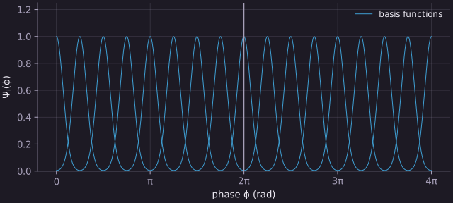
\[ \kbasis{\Psi_i(\phi)} = \exp\!\big(\kbasis{h}\,(\cos(\phi - \kbasis{c_i}) - 1)\big) \tag{38} \]
Read it aloud: bump \(i\) is largest, equal to 1, when the hand points at its center \(c_i\), and it fades smoothly away from there.
The centers \(c_i\) are spread evenly around the circle, and a larger width parameter \(h\) makes narrower bumps.3 Because of the cosine, a bump near the end of one lap joins the start of the next without a seam.
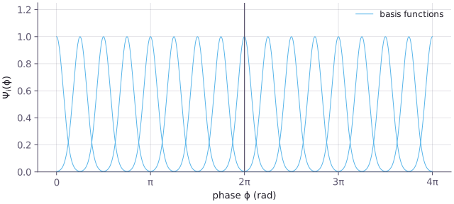
Learning the weights works as before: the recursive update (40)–(42) fits the weights one kernel at a time, and you will meet it in chapter 8.
Speed and size
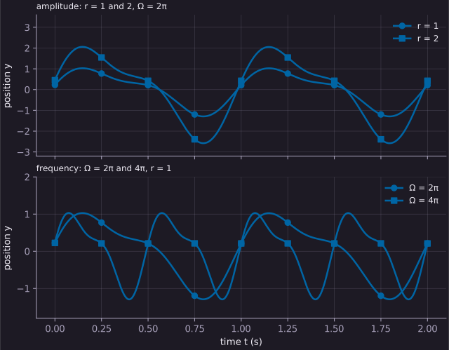
With the rhythm running, you can start turning the knobs: doubling \(r\) doubles the push, and the swing doubles along with it. Doubling \(\Omega\) sends the clock round twice as fast, so each lap takes half the time while keeping its shape.
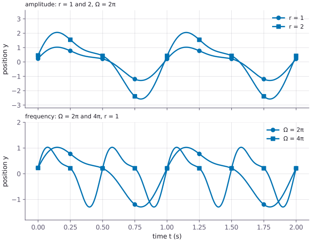
Moving the center
So far you have watched the rhythm swing around 0, because the spring in (34) has no goal and pulls toward \(y = 0\). That suits a wiper swinging around zero, but imagine an arm whose wave should be centered at 30°, rather than 0°.
Intuition: a spring that needs an anchor
Picture the arm tied to a post by a rubber band: in (34), that post stands at 0. For a wave centered at 30°, you need to tie the band to a post at 30°, so that moving the post carries the whole wave along. This post is the anchor, which we write as \(\kgoal{g}\).
The math: eq. (G09-6), (G09-8)–(G09-10)
\[ \dot{\kphase{\Phi}} = \kphase{\Omega} \tag{G09-6} \]
Read it aloud: the phase advances at the frequency, as before.
\[ \dot{\krepro{z}} = \kphase{\Omega}\Big(\underbrace{\kspring{\alpha_z\big(\beta_z(\kgoal{g} - \krepro{y}) - \krepro{z}\big)}}_{\text{spring–damper term}} + \underbrace{\frac{\sum_{i=1}^{N}\kbasis{\Psi_i}\,\kforce{w_i}\,r}{\sum_{i=1}^{N}\kbasis{\Psi_i}}}_{\text{forcing term}}\Big) \tag{G09-8} \]
Read it aloud: the spring now pulls toward the anchor \(g\), and the weighted push is scaled by \(r\).
\[ \dot{\krepro{y}} = \kphase{\Omega}\,\krepro{z} \tag{G09-9} \]
Read it aloud: the position follows \(z\), scaled by the frequency.
\[ \kbasis{\Psi_i} = \exp\!\big(\kbasis{h}\,(\cos(\kphase{\Phi} - \kbasis{c_i}) - 1)\big) \tag{G09-10} \]
Read it aloud: the bumps are the same circular bumps as before.
You have now met variant D2 from G09, and setting \(g = 0\) brings you back to (34).4 You may wonder whether the plain form can still learn a rhythm centered at 30°; it can, because the weights absorb the offset. That hidden offset becomes a problem later, once you change \(r\).
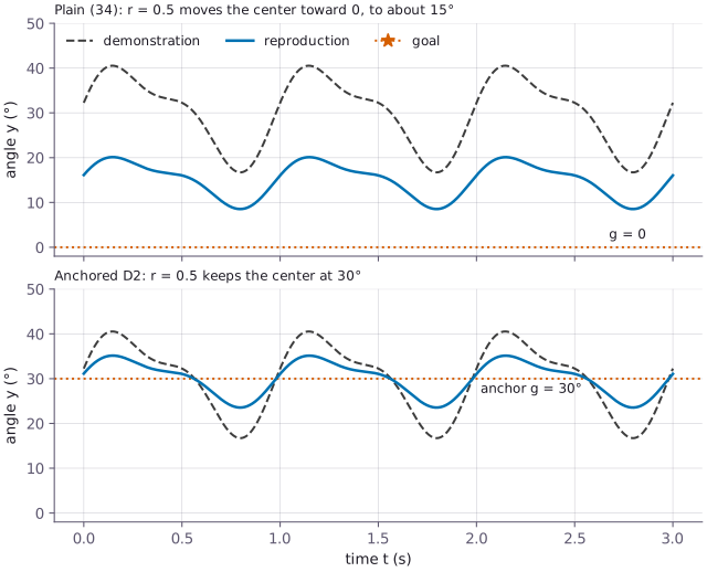
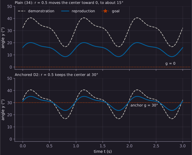
Drag \(\Omega\), \(r\) and the anchor \(g\) of variant D2, (G09-8), and watch which knob changes the speed of the swing, which its size and which its center.
In the plain form, the offset travels inside the push, so \(r\) scales it along with everything else. Giving the offset its own home in \(g\) lets \(r\) change only the swing.
Starting from rest
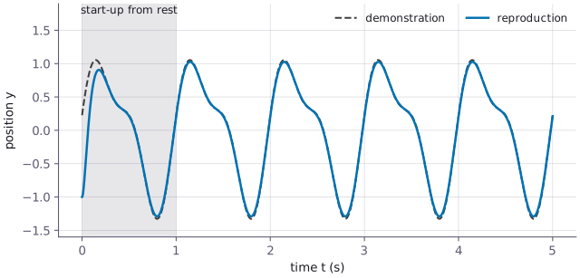
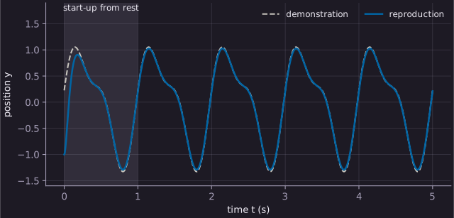
Before you rely on that steady rhythm, watch what happens when the robot starts at rest: its first lap looks different from the ones that follow.
Try it
Try it: 02_periodic_playground.ipynb › Simulate 2.4 - Omega, r and number of basis functions
As you drag \(\Omega\), the beat speeds up while its shape stays; try \(r\) for a bigger or smaller swing. Explore \(N\) to find how few bumps still give a good wave, then tick “start from rest” to watch its first lap wobble before settling. There is no slider for the center \(g\) here.
Try it: 03_create_your_own.ipynb › Create 3.4 - Define your wave
Here the arm waves around 30°, so you can move its anchor and watch the whole wave slide up or down while keeping its shape.
Gotcha
That wobble is a clue about what the robot learned: a rhythm to keep repeating, with no lesson for getting into it from rest.
Gotcha: the first laps are not taught
Symptom: the robot’s first cycles from rest differ from your demonstration. Cause: a classical periodic DMP learns the rhythm; the dynamics decide how it starts. S23 says it “does not encode the transient motion needed to start the periodic one” (p. 1143). This trips up everyone: a walking robot’s first step cannot be taught this way. Fix: start on the demonstration, the kit’s default, or allow a few warm-up laps before relying on the robot.