Chapter 5 · Learning from one demonstration
Show the robot a motion once, turn it into weights, and check how closely the robot can replay it.
Standing beside the robot arm, you take hold of its wrist as the motors go soft, then draw one smooth curve through the air from the shelf toward the box. The robot records every wobble, and when you let go, it replays that curve on its own, as smoothly as you drew it. This is kinesthetic teaching, a name for “teaching by moving the robot’s body,” and here you build the part that turns one recording into a motion the robot owns.
The picture
Imagine laying tracing paper over a drawing and following its lines once, until the shape belongs to your own sheet. You can return to that copy whenever you like and reproduce the drawing, even with your eyes closed.


A DMP keeps its own kind of tracing, storing a short list of numbers, the weights \(\kforce{w_i}\), from which it can rebuild the curve whenever you ask. The recording becomes those weights rather than a point-by-point copy.
The idea
We already have a spring to pull the robot toward the goal and a clock that fades from 1 to 0, so two parts of our machine are ready. What remains is the push \(\kforce{f}\), which has to bend the path into the shape you drew.
To find it, imagine asking the spring what push would have made it follow this exact demonstration. We can answer that question in two steps.
- At every recorded moment, work out the push the spring would have needed, giving us the target push \(f_d\).
- Then choose the weights so that the bumps, added up, match that target as closely as possible.
The math
Intuition: run the spring backwards
Usually you choose a push and watch the spring move; this time, you watch the motion and ask which push could have caused it. It is like following a ball through the air and working out how hard it was thrown.
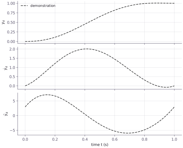
Your demonstration gives us positions \(\kdemo{y_d}\) recorded at sample times \(t_J\), and we also need its velocity and acceleration: the speed and the rate at which that speed changes. Differencing the positions gives us those quantities, although the built-in reach already comes with exact ones.1
The math: eq. (6)
\[ \kforce{f_d(t_J)} = \tau^2\,\kdemo{\ddot y_d(t_J)} - \kspring{\alpha_z\Big(\beta_z\big(\kgoal{g} - \kdemo{y_d(t_J)}\big) - \tau\,\kdemo{\dot y_d(t_J)}\Big)} \tag{6} \]
Read it aloud: the push needed at each sample is the acceleration (scaled by \(\tau^2\)) minus whatever the spring–damper term already supplies.
Think of equation (6) as equation (1) turned inside out: in (1) you put a push in and get a motion, while in (6) you put the motion in and get the push out.
You can follow the three signals going into (6) in the figure below, using the built-in reach as our demonstration.
By now we have a target value \(f_d\) for every sample, each one a number that our model for \(f\), the weighted sum of bumps in eq. (4), should match. Gathering all those samples together gives us one linear system for the weights.
Intuition: a recipe with N ingredients
Imagine each bump as an ingredient with a fixed shape, and its weight as the amount you pour into the mixture. We are looking for the amounts that make the finished mixture taste like the target.
The math: eq. (7)–(8)
\[ \boldsymbol{\Phi}\,\kforce{w} = \kforce{\mathfrak{F}} \tag{7} \]
Read it aloud: the matrix of bump values times the weights should equal the stack of target pushes.
\[ \boldsymbol{\Phi} = \begin{bmatrix} \dfrac{\kbasis{\Psi_1(x_1)}}{\sum_{i=1}^{N}\kbasis{\Psi_i(x_1)}}\,x_1 & \cdots & \dfrac{\kbasis{\Psi_N(x_1)}}{\sum_{i=1}^{N}\kbasis{\Psi_i(x_1)}}\,x_1 \\ \vdots & \ddots & \vdots \\ \dfrac{\kbasis{\Psi_1(x_{\mathfrak{T}})}}{\sum_{i=1}^{N}\kbasis{\Psi_i(x_{\mathfrak{T}})}}\,x_{\mathfrak{T}} & \cdots & \dfrac{\kbasis{\Psi_N(x_{\mathfrak{T}})}}{\sum_{i=1}^{N}\kbasis{\Psi_i(x_{\mathfrak{T}})}}\,x_{\mathfrak{T}} \end{bmatrix} \tag{8} \]
Read it aloud: row \(J\) of the matrix holds the normalized bump values at sample \(J\), each multiplied by the phase \(x_J\).
Picture the matrix as a table with one row per sample and one column per bump, with far more samples than weights to work with. No set of weights fits every sample exactly, so we ask NumPy for the least-squares answer: the weights with the smallest total squared miss. In dmpkit, one call to np.linalg.lstsq does that work.
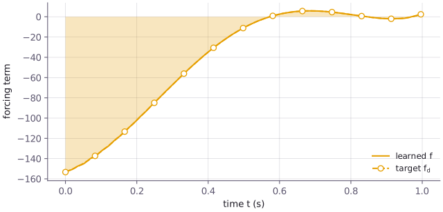
Before we send the spring on its way, let us compare the learned push with the target it was trying to match.
Then comes the check that matters for the robot: run the spring and learned push forward in time with explicit Euler (E4), and compare the motion with your demonstration.
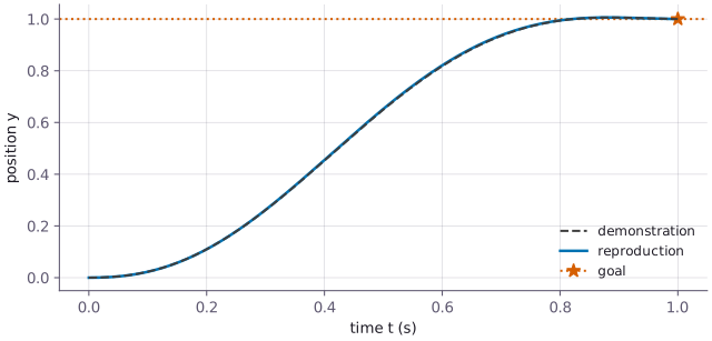
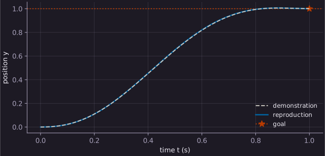
Step the number of bumps \(N\) from 2 to 60 and watch the solid replay close in on the dashed demonstration, and the gap in the readout shrink until it levels off at about 0.3 %.
The curves lie together, and the reach you drew is now a motion the robot can call its own.
Learning on the fly
The least-squares method we just used waits until the whole demonstration is available, which is why we call it a batch. But imagine the samples arriving one by one, with the weights improving as each new piece of the movement comes in.
Intuition: a running average, but for weights
Think of keeping a running average as new numbers arrive: instead of rebuilding the whole sum, you nudge the old answer by a fraction of the surprise. Recursive least squares carries that same idea over to the weights.
The math: eq. (9)–(10)
\[ \mathbf{P}_J = \frac{1}{\lambda}\left(\mathbf{P}_{J-1} - \frac{\mathbf{P}_{J-1}\boldsymbol{\varphi}_J\boldsymbol{\varphi}_J^{\top}\mathbf{P}_{J-1}}{\lambda + \boldsymbol{\varphi}_J^{\top}\mathbf{P}_{J-1}\boldsymbol{\varphi}_J}\right) \tag{9} \]
Read it aloud: after each sample, update the matrix \(P\), which tracks how sure the learner is about each direction, dividing by the forgetting factor \(\lambda\).
\[ \kforce{\mathbf{w}_J} = \kforce{\mathbf{w}_{J-1}} + \big(\kforce{f_d(t_J)} - \boldsymbol{\varphi}_J^{\top}\kforce{\mathbf{w}_{J-1}}\big)\,\mathbf{P}_J\boldsymbol{\varphi}_J \tag{10} \]
Read it aloud: the new weights are the old weights plus the surprise, the target minus the current prediction, steered by the matrix and the basis values at that sample.
We begin the recursion with \(P\) equal to the identity matrix and all weights zero, then let each arriving sample shape the answer. With a forgetting factor of \(\lambda = 1\), nothing is forgotten along the way.
After one sweep through the demonstration, though, the weights still differ from those found by batch least squares, as the paired bars below show.
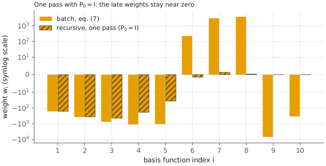
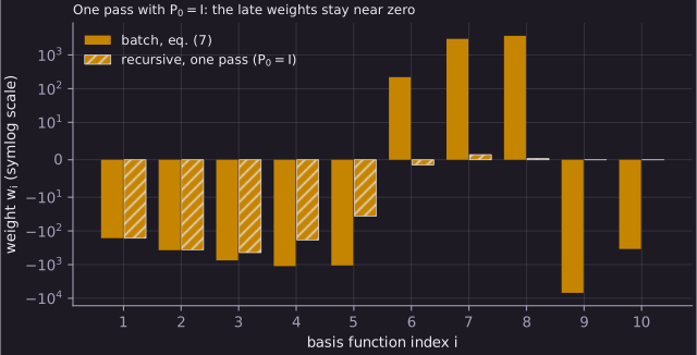
The difference begins with the start value \(P_0 = I\), which acts like a gentle pull of every weight toward zero. One pass of (9)–(10) therefore gives exactly the least-squares answer with that extra pull included. In eq. (8), every row carries the phase \(x_J\), and by the time the late bumps wake up, that phase is tiny. For those bumps the pull toward zero wins over the data, leaving their weights near zero while the first ones match the batch weights. More passes help, although slowly; with a much larger start, such as \(P_0 = 10^6 I\), we get the batch replay in one pass. This explains why the discrete notebooks use the batch version, and why the periodic DMP of Chapter 8 returns to the demonstration over many laps.
Try it
Try it: 01_discrete_playground.ipynb › Simulate 1.2 - Fit the demonstration and replay it
When you run this cell, it fits \(N = 30\) bumps to the demonstration and replays the movement. Follow the dashed demonstration and solid replay toward the star marking the goal, and look for the two curves lying on top of each other.
Try it: 01_discrete_playground.ipynb › Test 1.3 - How close is the replay?
Run this cell to put a number on what you saw: it prints the largest gap in percent of the motion’s size, with PASS appearing when the gap is under 5 %. Once you have checked the built-in motion, return to Create 1.1 - Choose a demonstration and set DEMO to "waypoints" with your own list of numbers. Now you can see whether your own curve passes too.
Gotcha
Gotcha: noisy demonstrations give wild accelerations
Symptom: the push \(f_d\) looks like static, leaving the replay jittery or wrong. Cause: eq. (6) needs the acceleration, so taking differences of positions twice turns even tiny measurement noise into a much larger signal (compare S23 Fig. 7, p. 1143, 10.1177/02783649231201196). Fix: smooth the demonstration before you differentiate it, so the noise does not overwhelm the motion you meant to teach. This trips up everyone the first time a real sensor joins the story.