Chapter 6 · New goal, new speed
Same weights, two new numbers: send the motion to a new goal, and play it faster or slower.
The robot arm learned its reach yesterday, and today the boss walks in: the shelf moved 20 centimeters, and the motion needs to finish in half the time. You can keep the weights from that one demonstration and give the arm its new task by changing two numbers: the goal \(\kgoal{g}\) and the time constant \(\kphase{\tau}\). Then press go; the robot needs no second lesson.
Let us follow what happens when you turn those two knobs, because one changes the motion just as you might expect, while the other holds a small surprise.
The picture
Picture signing your name across a whiteboard and then squeezing it onto a small form: the size changes, yet the handwriting stays recognizably yours. The same is true when you sign quickly at the checkout or take your time over a contract.


The weights hold the DMP’s version of that familiar “style,” the way your hand moves, while the goal chooses where the motion ends and the time constant sets how quickly it gets there.
Keep one detail of the signature picture in mind: your hand adjusts size and speed together without much thought, while a DMP needs a choice from you. Changing speed comes with the model; making the shape scale in size takes an extra ingredient.
The idea
Speed first. Let us start with the time constant \(\tau\) and the phase \(\kphase{x}\), the clock you met running from 1 down to 0. Because \(\tau\) sets how fast that clock ticks, a larger \(\tau\) slows it down, and the rest of the DMP follows along. The whole motion then plays back more slowly or quickly along exactly the same path in space.
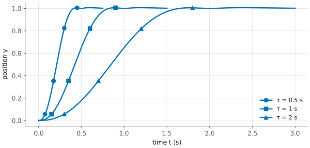
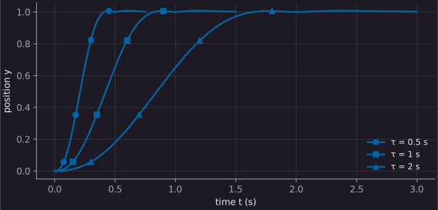
Goal second. Changing the destination asks something subtler of the model, because in the survey form, eq. (4), the forcing term is a fixed learned push whose formula never mentions the goal. The spring–damper term does know the destination and pulls toward the new \(g\), so the familiar push now travels with a different pull.
Imagine moving the finish farther away: the spring has more work to do, while the learned push stays the same size. The path still arrives because the spring wins in the end, but its shape looks flatter, with the same bump of push spread over a longer trip.
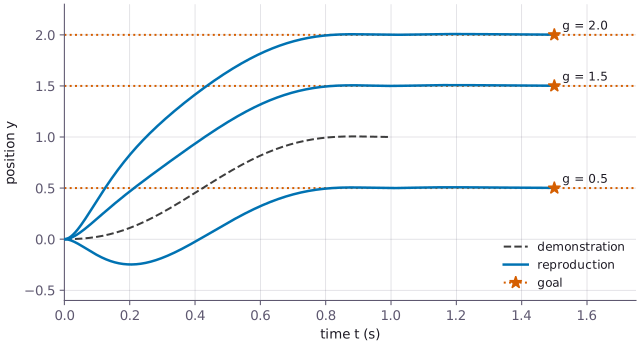
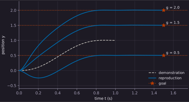
To make the shape grow with the trip, we can choose variant D1, which multiplies the push by the trip length, \((g - y_0)\), where \(y_0\) marks the start. A longer trip then brings a bigger push, stretching the shape like your signature across the whiteboard.
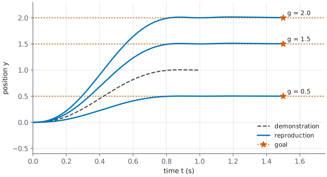
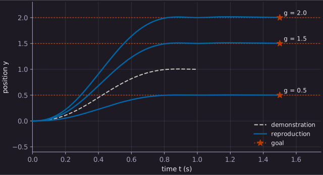
Drag the goal \(g\) and the time \(\tau\) and watch the replay follow; tick “scale by (g − y0)” to switch from the survey form (4) to variant D1, (IJ-2.3), and see the shape stretch.
Intuition: two knobs, two behaviors
Turning \(\tau\) feels like moving a video’s playback slider, watching the same picture unfold at a different speed. Turn \(g\) in the survey form, and the finish line moves while the runner keeps the same running style. Turn \(g\) in the scaled variant, and the runner’s stride stretches too, to fit the new track.
The math
The same equations are ready to take us to the new destination; we just put the new \(g\) and \(\tau\) into the model we already know.
Intuition: same machine, new settings
Picture the equations as a familiar machine with two dials on its side: you can turn those dials to change the motion without rebuilding what is inside.
The math: eq. (1)–(3)
\[ \kphase{\tau}\,\krepro{\dot z} = \underbrace{\kspring{\alpha_z\big(\beta_z(\kgoal{g} - \krepro{y}) - \krepro{z}\big)}}_{\text{spring–damper term}} + \underbrace{\kforce{f(x)}}_{\text{forcing term}} \tag{1} \]
Read aloud: the speed of \(z\), scaled by \(\tau\), is the spring pulling toward the goal plus the learned push.
\[ \kphase{\tau}\,\krepro{\dot y} = \krepro{z} \tag{2} \]
Read aloud: the speed of the position, scaled by \(\tau\), is \(z\).
\[ \kphase{\tau}\,\kphase{\dot x} = \underbrace{-\kphase{\alpha_x}\,\kphase{x}}_{\text{the clock runs down}} \tag{3} \]
Read aloud: the phase shrinks at a rate set by \(\alpha_x\), and \(\tau\) stretches that clock.
Look at \(\tau\) on the left of all three equations, and nowhere else: making \(\tau\) twice as big makes every change take twice as long. That stretches the journey in time while keeping its path in space. Meanwhile, the goal \(g\) sits only inside the spring term of eq. (1), so changing the destination leaves the weights untouched.
Intuition: the push is a fixed recipe
Think of the survey form as a recipe for the push, written once from the demonstration with no goal among its ingredients. A new destination changes the spring pulling the robot home, while the recipe keeps making the same push.
The math: eq. (4)
\[ \kforce{f(x)} = \frac{\sum_{i=1}^{N} \kforce{w_i}\,\kbasis{\Psi_i(x)}}{\sum_{i=1}^{N} \kbasis{\Psi_i(x)}}\; \kphase{x} \tag{4} \]
Read aloud: the push is a weighted blend of bumps, faded out by the phase, and no goal appears anywhere in it.
When you want the push to grow with the trip, the scaled variant D1 gives you that extra ingredient, as described by Ijspeert and colleagues (10.1162/NECO_a_00393, p. 333).
The math: eq. (IJ-2.3)
\[ \kforce{f(x)} = \frac{\sum_{i=1}^{N} \kbasis{\Psi_i(x)}\,\kforce{w_i}}{\sum_{i=1}^{N} \kbasis{\Psi_i(x)}}\; \kphase{x}\,(\kgoal{g} - y_0) \tag{IJ-2.3} \]
Read aloud: the same blend as in (4), now multiplied by the trip length \(g - y_0\), so a longer trip means a bigger push.
Choosing D1 also changes how we learn: the weights are fitted with the demonstration’s trip length, so each row of the learning matrix in eq. (8) is multiplied by \((g - y_0)\). When you replay the motion toward a new goal, that factor changes along with the destination.1
Try it
Try it: 01_discrete_playground.ipynb › Simulate 1.4 - Goal, start, tau and number of basis functions
Open this cell and move the goal slider \(g\), following the path as it reaches the new destination without another lesson. Then drag \(\tau\) and watch the same journey take more or less time, before ticking “scale by (g − y0)” to switch from the survey form (4) to the scaled variant (IJ-2.3). As you move the goal, look for the shape stretching with it, and try placing the goal below the start to see what each form does.
Gotcha
Gotcha: under the scaled variant, a goal near the start switches the push off
Symptom: after you tick “scale by (g − y0)” and place the goal very close to the start, the robot does almost nothing or moves in an odd way. Cause: the factor \((g - y_0)\) in (IJ-2.3) approaches zero when start and goal almost coincide, taking the push with it. Picture a tap on a table that begins and ends at the same height: there is no “trip” left to scale. IJ13’s fix, eq. (IJ-2.18), addresses a demonstration whose start and goal coincide by dividing by the trip length used in fitting, keeping the push on during learning. A goal moved near the start afterward still leaves \((g - y_0)\) as a factor, so this fix cannot help and can instead magnify the motion hugely (IJ13 pp. 346–347). Fix: for motions that begin and end at nearly the same place, choose the survey form (4), whose push has no factor \((g - y_0)\) to switch it off.