Chapter 8 · Teaching a rhythm
Learn a rhythm from a noisy recording, one lap at a time, and judge whether the robot really got it.
Take the robot’s hand and shake it up and down a few times, showing it the wave you would like it to learn. A camera catches every wiggle, including the noise, leaving the robot with a messy recording from which to find a rhythm it can wave back on its own.
In Chapter 7 you met the periodic DMP with weights the kit had already learned; now you will walk through the learning itself, from that noisy recording to the numbers behind the wave.
The picture
Think of learning a song by ear, humming along as the chorus comes round and missing most of the notes on your first attempt. When the chorus returns, the part that caught you out a moment ago sounds a little better, and after a few laps the tune begins to fall into place.


Along the way, you have to decide how much to trust your memory of the first lap compared with what you heard just now. Hold too tightly to the old laps and you never adapt; trust only the newest and one bad note can throw you off. A number called the forgetting factor \(\lambda\) sets that balance.
The idea
As in Chapter 5, we follow the recording with a question in mind: “What push would have produced this demonstration?” The answer is the desired forcing value \(\kforce{f_d}\), which we work out at every moment using the demonstrated position \(\kdemo{y_d}\), its velocity and its acceleration.
The acceleration is where that innocent-looking camera noise becomes troublesome, because taking differences of the positions twice makes the noise much larger. You can see the result in the figure below.
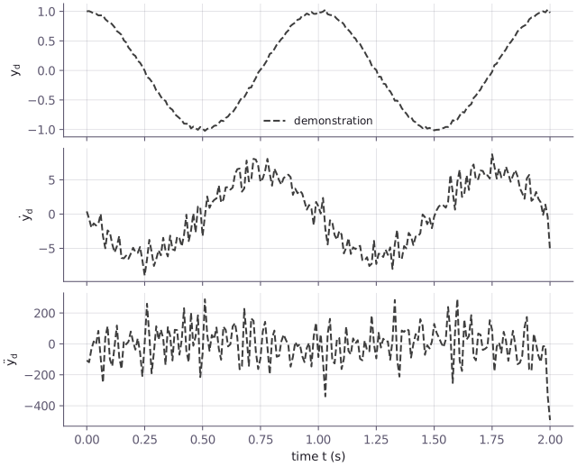
You do not have to chase every spike: each bump only needs to find the average push that fits its own part of the cycle.
Intuition: each bump keeps its own running guess
Imagine every bump \(\kbasis{\Psi_i}\) carrying its own number, the weight \(\kforce{w_i}\), along with a small gauge of how sure it is. As the phase passes over, the bump wakes up, compares the push the demonstration needs with the push it currently gives, and nudges its weight to close the gap. Far from the phase it sleeps and barely changes; it is the waking moments, lap after lap, that let each weight settle.
The math
Intuition: a target, an error, a nudge
Once you know the push the demonstration needs, subtract the push the bump gives now and use a fraction of the difference to nudge its weight. That is the learning step you will repeat along the recording.
Let’s begin with the push we need to explain: it comes from the demonstrated acceleration after accounting for what the spring alone would give.
The math: eq. (39)
\[ \kforce{f_d(t_J)} = \frac{\kdemo{\ddot y_d(t_J)}}{\Omega^2} - \kspring{\alpha_z\left(\beta_z\big(-\kdemo{y_d(t_J)}\big) - \frac{\kdemo{\dot y_d(t_J)}}{\Omega}\right)} \tag{39} \]
Read aloud: the push needed at sample \(t_J\) is the demonstrated acceleration, divided by the frequency squared, minus the pull the spring and damper already supply.
Now you can give each bump \(i\) its own weight and gain \(P_i\), the number that tells it how fast to learn. Before the recording begins, the gain starts at 1 and the weight starts at 0.
The math: eq. (41), (42), (40)
\[ e_r(t_J) = \kforce{f_d(t_J)} - \kforce{w_i(t_J)}\,r \tag{41} \]
Read aloud: the error of bump \(i\) is the push we want, minus the push its weight gives now.
\[ P_i(t_{J+1}) = \frac{1}{\lambda}\left(P_i(t_J) - \frac{P_i(t_J)^2\, r^2}{\dfrac{\lambda}{\kbasis{\Psi_i}} + P_i(t_J)\, r^2}\right) \tag{42} \]
Read aloud: the new gain is the old gain, shrunk a little by what was just learned, and divided by the forgetting factor \(\lambda\) so that old samples fade.
\[ \kforce{w_i(t_{J+1})} = \kforce{w_i(t_J)} + \kbasis{\Psi_i}\,P_i(t_{J+1})\,r\,e_r(t_J) \tag{40} \]
Read aloud: the new weight is the old weight, plus the error, scaled by how awake the bump is (\(\Psi_i\)), by the new gain and by the amplitude \(r\).
Keep the order close at hand: equation (40) needs the new gain \(P_i(t_{J+1})\) from (42), which means you must compute (42) before (40).1
As you move through the recording, repeat this learning step at every sample for every bump. You can find it in S23 §2.2.1, p. 1143 (10.1177/02783649231201196). Let the demonstration cover whole periods, so that every bump receives the same number of visits.
Watch the weights below as twelve bumps listen to four periods of a noisy cosine in one pass, each finding its part of the rhythm.
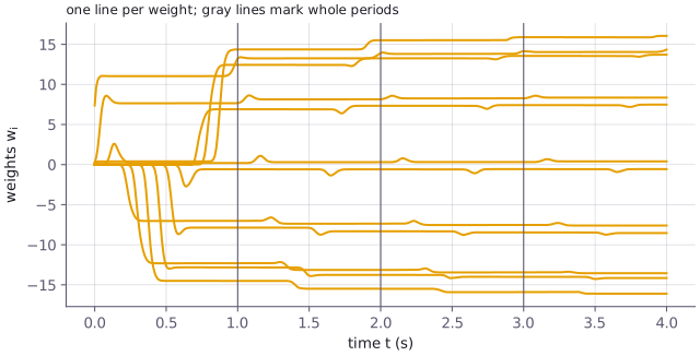
Once learning ends, you can put the recording aside and let the robot replay the rhythm from its learned weights alone.
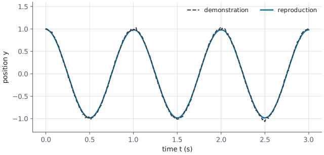
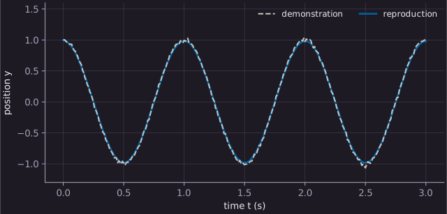
Follow the smooth solid path against the noisy dashed demonstration: for these two figures, the kit blurred the recording a little before taking derivatives, as the Gotcha of Chapter 5 advises. The bumps then averaged away the noise that remained, giving you a smooth replay through a learned weighted sum rather than a copy of every sample.
Try it
Now bring a rhythm of your own to the robot, and see how closely it can wave it back.
Try it: 02_periodic_playground.ipynb › Create 2.1 - Choose a rhythm
With RHYTHM set to "mine", you can write your own my_rhythm(t), a NumPy expression that repeats once per second. A sum of two sines gives you a place to begin; once it is ready, run the next cells and watch the robot replay your rhythm.
Try it: 02_periodic_playground.ipynb › Test 2.3 - How close is the replay?
When you run this cell on your rhythm, it prints the largest gap over three periods as a percent of the swing, and says PASS under 5 %. You can explore what the bumps can capture by giving the rhythm sharp corners and watching the gap grow, because a small collection of bumps cannot follow a sharp corner.
For another turn at the controls, try Create 2.5 - Challenge in the same notebook, where you can ask the robot to wave three times per second at twice the swing.
Gotcha
Gotcha: sleeping bumps can blow up the update
Symptom: with many narrow bumps, Python raises a ZeroDivisionError, or NumPy prints “divide by zero encountered” warnings. Cause: equation (42) divides by \(\Psi_i\), and far from a bump’s center \(\Psi_i\) becomes so tiny that the computer rounds it to exactly 0. The term \(\lambda/\Psi_i\) then blows up to infinity, a trap that trips up everyone. Fix: once \(\Psi_i\) falls below a tiny threshold, skip that bump’s update for the sample, because even a successful division would produce only a vanishingly small change. The kit follows this rule: a kernel whose \(\Psi_i\) is below \(10^{-6}\) sleeps.